Raster mapping example
1 Introduction
This RMarkdown document describes reading a netCDF file consisting of several bioclimatic variables, and plots one of them
1.1 Load packages
# load libraries
library(ncdf4)
library(CFtime)
library(lattice)
library(RColorBrewer)
2 Read data
# set path and filename
ncpath <- "/Users/jamie/Desktop/salt.anal1deg.nc"
ncname <- "salt.anal1deg.nc" ncfname <- paste(ncpath, ncname, ".nc", sep="")
class="s1">dname <- "salt"
# open a netCDF file
ncin <- nc_open(ncpath)
print(ncin)
## 1 variables (excluding dimension variables):
float salt[lon,lat,level,time]
long_name: Ocean Salinity, analyzed mean, 1-deg grid, Monthly
valid_range: 0
valid_range: 100
actual_range: 3.52430009841919
actual_range: 41.4294013977051
units: g/kg
add_offset: 0
scale_factor: 1
missing_value: -9.96920996838687e+36
var_desc: Ocean Salinity, analyzed mean
dataset: NODC World Ocean Atlas 1998
level_desc: Multiple Levels
statistic: Analyzed Mean
parent_stat: Mean
4 dimensions:
lon Size:360
units: degrees_east
long_name: Longitude
actual_range: 0.5
actual_range: 359.5
standard_name: longitude
axis: X
lat Size:180
units: degrees_north
long_name: Latitude
actual_range: 89.5
actual_range: -89.5
standard_name: latitude
axis:
level Size:24
units: meters
positive: down
long_name: Level
actual_range: 0
actual_range: 1500
axis: Z
time Size:12 *** is unlimited ***
units: days since 1-1-1 00:00:0.0
long_name: Time
actual_range: 0
actual_range: 334
delta_t: 0000-01-00 00:00:00
avg_period: 0097-00-00 00:00:00
prev_avg_period: 0000-01-00 00:00:00
ltm_range: 693597
ltm_range: 729026
standard_name: time
axis: T
2.1 Longitude and Latitude
# get longitude and latitude
lon <- ncvar_get(ncin,"lon")
nlon <- dim(lon)
head(lon)
## [1] 0.5 1.5 2.5 3.5 4.5 5.5
lat <- ncvar_get(ncin,"lat")
nlat <- dim(lat)
head(lat)
## [1] 89.5 88.5 87.5 86.5 85.5 84.5
print(c(nlon,nlat))
## [1] 360 180
2.2 Time
# get offset time
time <- ncvar_get(ncin,"time")
time
## [1] 0 31 59 90 120 151 181 212 243 273 304 334
# get tunits
tunits <- ncatt_get(ncin,"time","units")
tunits
## $hasatt
[1] TRUE
$value
[1] "days since 1-1-1 00:00:0.0"
# get nt
nt <- dim(time)
nt
## [1] 12
2.3 Salinity array
salt_array <- ncvar_get(ncin,dname)
dlname <- ncatt_get(ncin,dname,"Ocean Salinity, analyzed mean, 1-deg grid, Monthly")
dunits <- ncatt_get(ncin,dname,"units")
fillvalue <- ncatt_get(ncin,dname,"actual_range")
# get dimension of salt array
dim(salt_array)
## [1] 360 180 24 12
2.4 Cf and Timestamps
# convert time to CFtime class cf
cf <- CFtime(tunits$value, calendar = "proleptic_gregorian", time)
timestamps <- CFtimestamp(cf)
timestamps
## [1] "0001-01-01" "0001-02-01" "0001-03-01" "0001-04-01" "0001-05-01"
[6] "0001-06-01" "0001-07-01" "0001-08-01" "0001-09-01" "0001-10-01"
[11] "0001-11-01" "0001-12-01"
# get character-string times timestamps
class(timestamps)
##
 year month day hour minute  second    tz     offset

    1     1     1   1    0      0      0 00:00      0

  2     1     2   1    0      0      0 00:00     31

  3     1     3   1    0      0      0 00:00     59

  4     1     4   1    0      0      0 00:00     90

  5     1     5   1    0      0      0 00:00    120

  6     1     6   1    0      0      0 00:00    151

  7     1     7   1    0      0      0 00:00    181

  8     1     8   1    0      0      0 00:00    212

  9     1     9   1    0      0      0 00:00    243

  10    1    10   1    0      0      0 00:00    273

  11    1    11   1    0      0      0 00:00    304

  12    1    12   1    0      0      0 00:00    334
# parse the string into date components time_cf
time_cf <- CFparse(cf, timestamps)
class(time_cf)
## [1] "data.frame"
3 Plot the Data
# levelplot of the array
grid <- expand.grid(lon=lon, lat=lat)
cutpts <- c(3.7,11.1,18.5,25.8,33.2,40.6)
levelplot(salt_array ~ lon * lat, data=grid, at=cutpts, cuts=11, pretty=T, col.regions=(rev(brewer.pal(10,"RdBu"))))
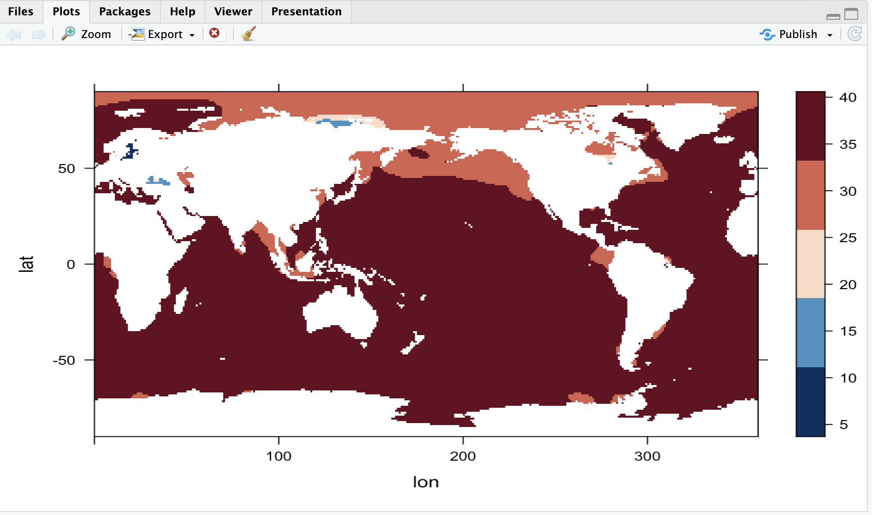
4 Discussion:
The image above shows the Salinity data around the globe in 1998.
The dark red represents areas with high amounts of salinity, and the dark blue represents areas with low amounts of salinity in the ocean.
The whites represent the areas that are the land and not the ocean.
Looking at the map, the first thing I noticed was that it looks like salinity in the water tends to be lower overall in areas that are at the top of the earth in the north.
My guess for this is because of the large amount of glaciers and frozen water there, the melting ice that turns into water dilutes the ocean making it less salty.
The only two areas that did seem to have low salinity levels even though they weren't high up north was the Baltic Sea and Black Sea.
My guess for this is because there are a lot a freshwater runoff from the surrounding land like rivers and streams that help dilute the salt in the ocean